ACKNOWLEDGEMENTS
The one person I must really
give a heart felt thanks to is Steve Foster, the I.T. manager at my school. He
is not only an I.T. guru, but also a physics teacher, programmer, researcher,
cosmologist, father and a great friend.
Regardless of work piling up on his shoulders like the Earth on Atlas’, Steve
would still be genuinely eager to make time and sit down with me, discuss my
ideas and share past experience in the field of astronomy and computing.
Steve has been one of the prime factors in the inspiration of this project,
helping me to clarify my direction and follow the project through to (partial)
completion.
I must also sincerely thank the entire staff of my school’s “I.T. Centre”, who
unfortunately did not enjoy the last holiday and have had to put up with me
throughout this past year (especially during the first few trials of my
modelling software).
Finally my local family: my mother at home, and my grandmother, who have
supported me every way they could in realising this endeavour that initially
seemed just outside of my grasp at this hectic point in my life.
02/09/2001
CONTENTS
·
Introduction
Part A –
Research:
1.
A
Simple Model
o
The
Interstellar Medium
o
Collapse
o
Observations
and Predictions
2.
Complications
o
Fragmentation
and Rotation
o
Magnetic
fields and Outflows
o
Galactic
links: Shockwaves and Self-sustaining formation
3.
Recent
theories
Part B –
Modelling:
1.
Definition
of the Problem
2.
The
Software
3.
The
Model
·
Conclusion
·
Bibliography
INTRODUCTION
As
we lead our busy day-to-day lives on this planet – attending to a multitude of
everyday endeavours – it would be fair to say that we give very little
consideration to our astronomical origins. As absurd it may seem, our origins
lie in a sequence of cosmological processes that began billions of years ago.
They finally allow for our ability to contemplate this notion (and our very
existence).
These
particular ‘cosmological processes’ range in scale and expression, and are on
the whole not well understood despite the substantial advances made in the last
few decades. For a moment let us view the big, big picture. Apart
from the Big Bang – the moment our universe came into existence (which we
should take for granted here so as to avoid the headache of the quantum
‘froth’) – these processes have transpired with what appears to be mechanical
precision.
The Strong and Weak Anthropic Principles
find their foundation in this notion: whether the chances of ‘everything going
right’ from the outset was a mere fluke of ‘astronomical’ proportions, or that
our awareness of our home in the cosmos is a direct result of the fact that
everything did go right anyway. The question of whether the universe is
guided by any supernatural phenomena presents an entirely different ballgame,
but for the time being the project will attempt to examine issues from within a
framework provided by known physical laws and natural phenomena.
Let
us consider snapshots of the cosmological processes as a series of universal
events. One of the common phrases heard at someone’s burial is “ashes to ashes,
dust to dust”. Although it is a time of mourning and sadness, and not a good
opportunity to take a reductionist line of thinking, it is nevertheless
reassuring to realise that this ‘dust’ of which a person is made – the protons,
neutrons and electrons (and perhaps other exotic matter) originated in the Big
Bang, our first snapshot. During the cosmological processes that have occurred
over the past 8-15 billion years,
matter and energy have combined in just the right proportions with just the
right forces to construct what we see and feel at this moment.
The
more complex particles – which have been formed from the primary constituents
of the early universe following the Big Bang, hydrogen and helium
– were (and still are) being fused together inside the infernal factories of
billions of billions of stars
scattered throughout the cosmos. The super-massive stars quickly run out of
hydrogen as their main source of fuel and resort to ‘burning’ increasingly
heavier elements in other fusion reactions. Once a star begins to collapse
(being unable to sustain the inward gravitational pull with its radiation
pressure) it rapidly implodes, then explodes into a brilliant supernova,
lighting up the sky and more
importantly spewing vast amounts of the heavier elements back into the universe
that may be re-processed by other smaller stars, such as our Sun.
Now
let us imagine a snapshot of the birth of our Sun: the flash of the triggered
fusion reaction helps blast away the surrounding gas and dust revealing the
sparkling new orb. We can see much circumstellar dust and some largish chunks
of matter floating around the core. This is the birth of our solar system. The
largish ‘planetesimals’ are the foundation of proto-planet formation
and have appeared because heavier particles and dust grains have been
coagulating for some time around the ‘proto-Sun’. The particles eventually
build up in size, like a snowball, after incessantly bombarding each other,
slowly becoming more massive objects orbiting the Sun in roughly the same
plane. As the planetesimals collide to form proto-planets and the proto-planets
collide in enormous explosions, our planets take shape – their
composition is not of hydrogen and helium, but of the heavier elements
originally formed inside stars and simple compounds. As the system evolves and
the planets cool off from the heat of their forging, the conditions on one
planet just happen to be ideal for the formation of simple life forms, evolving
from complex molecular structures. Then, moving our snapshot forward again
several billion years, we arrive in the present day. When put in the
perspective of the universe, life on planet Earth seems utterly amazing.
However, life as we know it only orbits one star. There are billions of billions
of other stars ‘out there’ – might not life be too?
It
is this project’s aim to examine stars, in particular their formation. In
recent times much emphasis has been placed on larger and larger scale
structures, rather than their building blocks. Although we can look into the
night sky and see a multitude of stars, little of the precise details
are actually well understood about stellar formation. In the more recent past,
there has been much debate and conjecture about stellar formation, with many
theories and ideas being advanced that suggest interactions of dark matter and
changes in the development of stars now, in the visible universe, compared to
early times.
This
project will review the theories regarding the conditions and processes that
lead to star birth, how formation impacts on other ‘stellar nurseries’ and on
the formation of galaxies (a topic which is even less soundly understood), and
will discuss the creation of a basic model that investigates the possibilities
of stellar formation, based on altering initial conditions and physical forces.
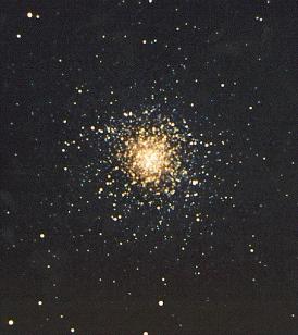
The star cluster of M13 – a
product of grouped
stellar formation from the
same massive matter cloud.
A SIMPLE MODEL – The Interstellar Medium A-1
As
we have observed that stars have long life times (in the range of a few million
to several billion years) and we believe the universe to be approximately 10
billion years old, it is safe to assume that not only did stars form in the
very early stages of the universe (as astronomers think old Population II stars
did)
but that stellar nurseries have existed ever since these early stages and star
formation is still active in the visible universe.
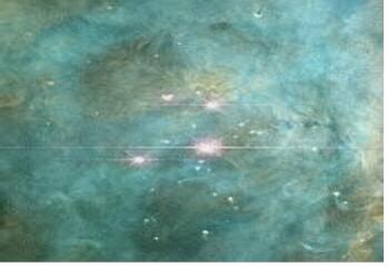
Today’s closest centres of star formation 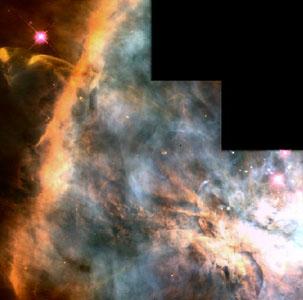 have been captured in vivid (false) colour by
optical telescopes, such as the Hubble Space Telescope and radio arrays, such
as the Very Large Array in the United States. Perhaps the most notable area of
star formation is the Orion Nebula. The image to the right is a portion of the
nebula (also known by its Messier Catalogue code: M42) photographed by the HST
– several optically ‘reddened’ stars, colourful dust and ionised gas regions
are visible. Both optical and radio images reveal such vast clouds of gas and
dust inside nebulae – clouds that are host to the birth of new protostars.
have been captured in vivid (false) colour by
optical telescopes, such as the Hubble Space Telescope and radio arrays, such
as the Very Large Array in the United States. Perhaps the most notable area of
star formation is the Orion Nebula. The image to the right is a portion of the
nebula (also known by its Messier Catalogue code: M42) photographed by the HST
– several optically ‘reddened’ stars, colourful dust and ionised gas regions
are visible. Both optical and radio images reveal such vast clouds of gas and
dust inside nebulae – clouds that are host to the birth of new protostars.
But
how do stars actually form? How does a system evolve to the stage of producing
a protostar? Although little has been understood about the subtleties of
stellar formation, there is one ‘overarching’ theory that is generally accepted
as the most plausible process. In its simplest form, it is the collapse of
clouds of matter that contract until a point is reached where enough heat is
generated to ignite fusion reactions. However even this simple model has its
own complexities.
These
matter clouds are the essential constituents of the InterStellar Medium (ISM)
and require a close study to fully understand stellar formation. The majority
of the ISM is showered with primary cosmic rays and is threaded with magnetic
fields.
The component gas and dust clouds are found distributed out over vast areas in
clumps.
The larger clouds tend to become the stellar nurseries that are home to new
stars (some of which are binary systems, super-massive stars and others that
will develop planetary systems).
It
is important to note the nature of this ‘simplistic’ theory. The processes to
be described here are those that seem to apply to stellar formation occurring
in the visible universe – formation whose building blocks are the matter clouds
of the ISM, a product of continual evolution, processing, recycling and
condensation over extended time periods. The processes that gas and dust clouds
underwent in the early “Dark Ages” of the universe might have been somewhat
different. Wondering what the building blocks of stellar formation were during
that era can raise the question of uncertainty in the current model’s
applicability: if there was no ISM as we observe today, what exactly
were the building blocks and formation processes of the early stars that formed
along side galaxies? A detailed answer still remains a mystery, although a
short discussion will ensue toward the end of Part A of the project.
Considering
only the gas found in the ISM for the moment, the element of highest abundance
is neutral hydrogen (H I) that tends to mass into large clouds. Other
components of the gas such as ionised atoms, free electrons and molecules, are
also present in varying smaller concentrations depending on their location. The
neutral hydrogen gas is cold (10-100 K) and extremely tenuous: at some points
the ratio of the distance between two atoms to their size is estimated12
to be 100 million to 1. For a hydrogen atom that is about 10-10
metres in diameter, such a ratio would mean its nearest neighbour would be
around 1 centimetre away.
Despite these comparatively large average distances between atoms of the gas,
the sheer volume and total mass of a cloud is enough to make it ‘clump’ and
sometimes develop stars.
The
gases between the H I clouds are also dilute but composed of mainly
ionised hydrogen (H II). They are hot and luminous as they interact with
radiation being emitted from nearby young O- and B-class stars. A typical H II
gas region is thought to surround these stars to a diameter of a few light
years. The hot stars (with a surface temperature of about 30 000 K) at the
centre of the cloud emit radiation at high enough energies (ultraviolet
photons) to ionise H I to H II increasing its temperature to about 10 000 K.
The basic equation for this reaction is:
H + UV Photon à H+ + e-
As
the ionised H II heats up it expands back into the cooler H I clouds while
forcing some more H I into its place. It is thought this process can influence
such clouds out to a distance of a few tens of light years. The image to the
right represents this phenomenon.
The
ionised H II regions are clearly visible as ‘fuzzy patches’ in many diffuse
(bright) nebulae in the night sky. As previously mentioned, the
Orion Nebula (about 20 light years in diameter) shows perhaps the best example
of these properties of the interstellar gas at optical and radio wavelengths. H
I has a characteristic 21-cm emission line (know as the Hydrogen-a line) that can be received by radio
telescopes. The emission spectrum of H II on the other hand, is continuous
(has a constant intensity over a range of wavelengths, as opposed to the
discrete peak or trough in emission or absorption line spectra). It is
continuous because an electron in an ionised atom, which will emit a photon,
can fall to any number of energy levels inside an atom – not just the ground
state – thus the photon has a wider set of possible frequencies (although the
individual wavelengths are quantised). This is known as the free-free emission
process and it enables radio astronomers to estimate the total mass of ionised
hydrogen atoms in an H II region (for example Orion which has about 300 solar
masses of H II gas).
The
existence of the H I clouds in the ISM was predicted by astronomers but not
observed until 1951 when radio telescopes picked up the 21-cm emission line of
neutral hydrogen. Surveys of nebulae, such as Orion, provided direct evidence
to show that the vast majority of the gas in most bright nebulae is infact H I.
Initially though, the H I regions could not be directly observed as they are cold
and not optically visible: the electrons in neutral hydrogen would barely ever
have enough energy to be promoted from the ground state to higher energy levels
– except when an atom would absorb ultraviolet light. However these UV
absorption patterns are not visible from ground-based telescopes as UV light is
hindered from penetrating the Earth’s atmosphere. It was with the advent of
satellite observatories, which could be situated outside the Earth’s
atmosphere, that the UV absorption spectra of H I clouds could be clearly
discerned.
The
UV images showed that the H I distribution in clouds of the ISM was ‘patchy’
ranging in diameters of about tenths of light years to tens of light years. The
average concentration of H I atoms in these clouds is thought to be
approximately 106/m3. Some regions have been shown to
have around ten times less per cubic metre. For comparison there are about 1025
particles per cubic metre in the air at the Earth’s surface. When looking at
our own Milky Way, H II is found to be concentrated in the plane of the galaxy.
Here an estimated concentration of 3x10⁵/m3 is found to
have a temperature of about 70 K. Again, for comparison there are about 1023
times more hydrogen atoms in one human body than there would be from this H II
concentration for the same volume. In total, H I clouds are supposed to make up
40% of ISM’s mass (each individual cloud being approximately 50 solar masses)
while H II clouds contribute very little.
The
elemental composition of interstellar gas does not only include neutral and
ionised hydrogen, but also to a lesser degree oxygen, nitrogen, sodium,
potassium, ionised calcium and iron. These elements have been found through
optical spectroscopy and have been confirmed as definite components of the gas,
not of the atmospheres whose stars emit the original photons. Interestingly,
strong evidence was provided for this claim while observing binary star
systems. As the stars orbit around one-another, their changing velocities shift
the absorption spectra of their atmospheres according to the Doppler effect
(hence they are called “spectroscopic binaries”). However the spectra of the
other elemental components of the interstellar gas were seen to remain still,
indicating they were not part of the stars.
There
exist cold molecular clouds in the ISM as well. They are found in close
proximity to active H II regions and exhibit a very wide range in total size.
The molecular clouds too contain mostly hydrogen, although it is in diatomic
form. Matter in these clouds is on the whole cold and easily observable at only
millimetre wavelengths. A search, started in the 1960s with the wide-scale
advent of radio telescopes, has revealed that there are over 60 different types
of molecules in the normal ISM: the majority are of an organic nature (contain
carbon atoms). The most common organic molecule is carbon monoxide (CO) and it
is accompanied by water, ethanol, ammonia, formaldehyde and free radicals of
hydrocarbons. The conglomerations of these molecules tend to form clouds near the
H II regions and sometimes result in several ‘cloud complexes’. These complexes
contain on average a few hundred molecules per cubic metre, are a couple of
tens of light years across and internally contain multiple molecular clouds of
different compositions, sizes and densities. The internal clouds have a density
of a few billion molecules per cubic metre and are held together by
their own gravity (for example those observed in Orion). Molecular clouds are
estimated to contribute a few billion solar masses (40%) to the ISM. An
individual cloud may have a mass of 103 solar masses while a cloud
complex may be about 104-107 solar masses. The cores of
sub-clouds in cloud complexes are vital to stellar formation as shall be seen
shortly. The temperatures inside sit around 10 K due to radiative cooling from
their ‘shells’. It is these self-gravitating cores that inevitably begin
collapsing and become the progenitors for new stars.
Apart
from interstellar gas clouds there are also inter-cloud regions. Ultraviolet
observations have provided direct evidence showing this gas to be very hot and
thin. The absorption spectrum of ionised oxygen atoms (O VI) has been found in
such regions, signifying that temperatures must be at about 106 K
(the temperature of the Sun’s corona – hence the inter-cloud gas is named the
‘coronal interstellar gas’). The gas is speculated to occupy 0.1% of ISM by
mass.
In
addition to all of these gases, the ISM contains dust (though it is incredibly
scattered). On average there is one dust particle for every million cubic metre
volume of space, yet the ‘grains’ contribute as much as several hundred solar
masses (1%) to the total mass of the ISM. Dust clouds can vary in size from
some 200 light years to a fraction of a light year. Some ultra-small clouds,
known as Bok globules measure one light year across and are so dense their mass
can reach 20 times the Sun15.
Dust
clouds provide stunning images of light extinction (the dimming of
starlight, for example the Horsehead Nebula) and reddening (the
scattering of wavelengths – most noticeable when increasing from the blue end
of the spectrum). Starlight
in the Milky Way is dimmed by a factor of 2 roughly every 3000 light years.
Dust clouds can also simulate the appearance of H II regions in bright nebulae
by simply reflecting the light from its host nebulae’s stars. Such reflection
nebulae do not exhibit the characteristic emission lines of an active H II
region, only an absorption spectrum of the stars whose light the dust clouds
reflect. The stars appear to be redder than the standard colour that would be
obtained from their spectral class analysis, as red light penetrates dust
clouds to a greater extent than blue light. This is because their blue light is
being preferentially scattered and absorbed (the principle behind the reddening
of the sun and moon as they sit on the horizon). The blue light that is not
absorbed is reflected inside the dust cloud until the photons leave in any
other direction. Thus the entire dust cloud itself takes on a bluish appearance
(as the sky here on the Earth does for the same reason). Dust leaves its
signature on background starlight as well: grains tend to be aligned along
extensive magnetic fields so that certain wavelengths of light are absorbed
depending on the orientation. By measuring the change in polarisation and thus
the alignment of the dust, it may even be possible to plot the directions of
the influential (though weak) Galactic magnetic fields.
 Despite dust’s curious nature, it provides
endless hassle to optical astronomers when it essentially blocks out the
visible light emitted from objects lying behind a dust cloud. Apart from
regions where extinction due to dust clouds is obvious as they form a defined
silhouette over a much brighter background (such as a large H II region), it is
nearly impossible to tell areas that are ‘clothed’, rendering that patch of sky
optically dark. However in this case, Infra Red astronomy comes into its own:
not only do IR photons penetrate dust clouds, the dust grains themselves can
act as tiny blackbody radiators re-emitting any absorbed radiation in the far
IR range of the spectrum when their temperature reaches about 100 K. So
although the optical peak from bright nebulae might lie in an active H II
region, the IR peak may lie elsewhere: in an IR cluster of cool dust near a
molecular cloud that is being heated by an external source. Such a difference
in peaks of separate spectral ranges is most apparent between the optically
strong source of the dense H II region in the Trapezium Cluster (the four stars
seen in the image on the right) and the strong IR core of the
Becklin-Neugebauer object behind it (thought to be powered by a massive
developing star), both in the Orion Nebula.
Despite dust’s curious nature, it provides
endless hassle to optical astronomers when it essentially blocks out the
visible light emitted from objects lying behind a dust cloud. Apart from
regions where extinction due to dust clouds is obvious as they form a defined
silhouette over a much brighter background (such as a large H II region), it is
nearly impossible to tell areas that are ‘clothed’, rendering that patch of sky
optically dark. However in this case, Infra Red astronomy comes into its own:
not only do IR photons penetrate dust clouds, the dust grains themselves can
act as tiny blackbody radiators re-emitting any absorbed radiation in the far
IR range of the spectrum when their temperature reaches about 100 K. So
although the optical peak from bright nebulae might lie in an active H II
region, the IR peak may lie elsewhere: in an IR cluster of cool dust near a
molecular cloud that is being heated by an external source. Such a difference
in peaks of separate spectral ranges is most apparent between the optically
strong source of the dense H II region in the Trapezium Cluster (the four stars
seen in the image on the right) and the strong IR core of the
Becklin-Neugebauer object behind it (thought to be powered by a massive
developing star), both in the Orion Nebula.
In
spite of the breakthrough in IR observations providing this new ‘visibility’ of
dust clouds, the accurate makeup of the individual dust grains eludes
astronomers. At first it is easy to select the most probable candidates from
the elements common to the ISM. Based on observations of light extinction and
reddening caused by dust, astronomers have formed a well-founded model that
suggests the grains have a small core about 0.05mm
in radius and a surrounding mantle layer about 1.0mm wide. The core is thought to be made from
silicates (supported by some recognised absorption patterns), iron or graphite,
and the mantle from a mixture of ‘icy’ materials (for example: water, carbon
dioxide or methane, which are solids below 100 K). It has been put forward that
the organic compounds of the mantle may have been ‘processed’ in reactions
offset by the ultraviolet light that permeates the ISM, forming more complex
molecules (much like in hydrocarbon substitution reactions).
Their precise composition is unknown too, though one theory proposes they are a
form of ‘tar’ that adds a considerable mass to each grain. The organic
processing of these molecules plays a crucial role in the formation of
molecules in molecular clouds. These two cloud types are closely linked: they
are usually found to inhabit each other’s space. The grains form a surface on
which molecules can build. For example: it is suggested that hydrogen atoms
readily ‘stick’ to a grain’s mantle in waiting for a collision with another
hydrogen atom. As they meet on the grain, a molecule of hydrogen will form.
Molecules cannot remain on the grain as easily, so it departs back into the
molecular cloud. The formation of larger molecules on dust presents a problem
with their ‘departure’ from the grain: they can easily split back up into their
component atoms. This has lead astrochemists to believe that although some
molecules may indeed form on mantles, molecules of up to around four atoms
could simply build up inside the gases of a molecular cloud by way of UV
catalysis and collision (not on a dust grain). Even though UV radiation
effortlessly breaks apart simple organic molecules, the construction of them
from single atoms is supposed to be ‘shielded’ from UV photons in the cores of
molecular clouds by other larger and more stable molecules.
The
formation of cosmic dust has been a puzzling phenomenon too. Cool giant and
M-class supergiant stars blow large amounts of mass into the surrounding space.
Denser dust grain cores are thought to form in the atmospheres of supergiants,
which are subsequently blown into the ISM. Their atmospheres would typically
peak at 2 500 K, allowing for hotter gases rising from within the star to
condense into small solid grains. The rate of total mass released is estimated
to climb as high as 10-5 solar masses per year. The smaller giants
release less: 10-6 solar masses per year. Observational evidence has
been found that supports this formation method by highlighting the unique
spectral characteristics of carbon and silicates in some stars’ atmospheres and
circumstellar clouds. The M-class stars that do have such circumstellar clouds
loose mass at the greatest rate of all: 10-4 solar masses per year –
they are thought to be the largest contributors to the ISM.
As
for the dust’s mantle, it is thought to condense inside dense, low temperature
molecular clouds. As a grain’s mantle only exists at low temperatures, when it
is heated to a couple of hundred kelvins, its mantle will evaporate. However,
it will ‘grow’ another every 108 years or so (the sheer number of
dust grains make this a regular occurrence).
The
application of infrared astronomy in the study of dust clouds has begun to
break down the optical barrier that obscures our view not only of other
galaxies and clusters, but also of areas of stellar formation. Since dust
contributes significantly to overall cloud volumes in the ISM, they partially
draw a curtain over the processes leading to the birth of new stars – in the
optical range. With past infrared observations (primarily using the Infrared
Astronomy Satellite, IRAS) dust cloud distribution and dynamics in the Milky
Way have been better comprehended. This knowledge can then be applied to
understand stellar formation processes. With the future launch (scheduled for
December 2001) of NASA’s fourth edition to the Great Observatories: the Space
Infrared Telescope Facility, SIRTIF,
astronomers can begin to uncover further mysteries of current stellar nurseries
using more sophisticated equipment to probe through these dusty ‘cocoons’.
A SIMPLE MODEL – Collapse A-1
It
is essential to realise that all models of stellar formation are in part
based on theory and there has yet been no compelling direct evidence to
support any definite sequence of events. Even a simple model founded on basic
collapse may well be missing critical undiscovered physical effects that play a
part in governing the evolution of protostars. This consideration of a “simple
model” here will discuss the overarching ideas of basic theoretical models:
cloud collapse, protostar development, and the accretion and dispersion of
matter.
The
process begins with the vast structures of matter clouds in the ISM. As a cloud
progressively builds in size and maintains a low temperature, these
self-gravitating regions will fall under the influence of gravity and begin to
collapse on themselves (not necessarily in the positional centre of each
cloud). It was Sir Isaac Newton who created the first mathematical description
of the force responsible for this very action
– although now it had been clarified as the curvature of space-time (Albert
Einstein’s revolutionary perspective of the universe). The cloud must be
sufficiently cold so the radiation pressure exerted by energetic particles does
not counteract the gravitational forces in the early stages. As the collapse
starts to accelerate, the rate of collapse at different points changes so the
cloud density should be dramatically different at various points. The central
regions of the cloud contract faster than the outer layers, which effectively
form an envelope around a condensing core. Once the core has formed and become
sufficiently hot it begins accreting the in-falling envelope. At this stage the
process may take either of two slightly different paths depending on the
initial mass of the collapsing cloud:
If
the original cloud was a ‘solar-mass cloud’ (i.e.: its total mass was around
that of one solar mass) and a few light years in diameter, it will form one
primary core that will develop into a protostar about twice the size of the Sun
typically in about 1 million years. While the central region is contracting
faster than the external layers, the pressure and density increase as
gravitational potential energy is converted into the kinetic energy of particle
collisions. The hydrogen molecules become the most active particles, and as
they collide with dust grains, the dust takes away some of the energy and
radiates it away at infrared wavelengths. This helps prevent – for a period –
the core from reaching excessive temperatures (a very high density and
pressure) that would slow down the inward pull of gravity with the opposite
push of radiation pressure. However given enough time the core will reach
critical density and become opaque to the radiation. This state is exacerbated
by the continual shower of in falling matter from the cloud’s external
envelope. As the temperature reaches about 2 000 K, hydrogen molecules split
into single atoms and serve to absorb enough radiation so that gravity may
continue with its inward haul – the increase in radiation pressure is too slow
to counteract gravity for the entire duration of this development. The
semblance of a protostar begins to contract again until the internal pressure
stabilises the gravitational force once more. Thus a protostar is born.
Although its luminosity is a few times that of our Sun, it is still shrouded in
the in-falling envelope and so blinded from the view of the optical astronomer.
The intense temperature does in fact heat the envelope up so much that it emits
strong infrared radiation. Such a compact source is thought to be the telltale
signature of stellar formation, especially when it comes from dense regions in
the ISM. The envelope will slowly dissipate leaving a shining cool
pre-main sequence star. The dissipation is though to occur not so much because
the majority of the envelope fall has fallen onto the protostar, rather that
the accretion flow has been reversed by strong solar winds generated by the
star. The envelope is blown away from the core as the star recycles the
remaining portion of its share of the ISM for other future stars to use. Until
its ‘star-hood’, the majority of emitted radiant energy will come from the
release of gravitational energy. An estimated 50 million years passes before a
protostar properly matures and joins the main sequence. At this moment the
concentrated bombardment of particles inside the protostar’s core gives way to
ignition of nuclear fusion reactions
while the accretion of the envelope draws to a close.
If
the mass of the original cloud was not in the order of solar masses but much
greater, a massive protostar forms in a similar sequence of events. The main
difference is that after an estimated 300 000 years, the core becomes hot and
dense enough to initiate fusion reactions before accretion of the
envelope reaches an end. At this point, around half of the original cloud mass
found in the envelope is blown back into the ISM, a great proportion more than
solar mass protostars. The new massive protostars are also more luminous and
thus stronger infrared sources. In addition, the fusion reactions produce
copious amounts of ultraviolet photons that ionise the circumstellar gas
transforming it into another H II region, which helps in the dissipation of the
remaining envelope too. The high output of UV and IR radiation makes massive
protostars more easily identifiable in space. Understandably many more massive
protostar candidates have been found in the sky than solar mass ones. The
quicker evolution of massive protostars allows them to reach the main sequence
long before their solar-mass counterparts, even though they appear to still be
shrouded in the remnants of their dusty molecular host cloud.
An active stellar nursery
A SIMPLE MODEL – Observations and Predictions A-1
Much
speculation still exists over the formation of solar-mass stars, as they are so
much smaller than massive protostars. On the other hand the birth of massive
stars seems to appear with a possible set of known radiation emissions in
different spectral bands dependant on the protostar’s progress. The following
is a prediction of the likely sequence of events based on observational
evidence:
After
about 300 000 years as young massive protostars begin shinning from the
gravitational contraction of a massive molecular cloud, they should appear as a
compact far-infrared sources linked to their parent cloud. Some theory suggests
massive stars that finish accreting matter early should be metal poor.
Throughout the next 50 000 years as their surface temperatures increase while
fusion burning ignites in their cores, the protostars are now observed as
near-infrared sources. During the following 30 000 years as nuclear reactions
proceed, emitted ultraviolet photons create a new H II region around the stars,
enabling their detection as a strong radio emission source. The H II regions
expands in size at about 5-10km/s for 500 000 years while infrared emission
strength decreases (while the protostars’ envelopes begins to dissipate). At
this point the H II regions are optically visible and emit radiation of
centimetre-radio wavelengths. For the next 2 million years both the H II
regions and parent cloud dissipate. Infrared emissions drop off and radio
signals become diffuse. By now, several new O- and B-class stars have
materialised from the once massive molecular clouds. The important fact to
realise here is the preceding section, describing the collapse of matter
clouds, dealt with single stars; stellar formation is thought typically to
occur in associated clusters. After a subsequent 6 million years, H II regions
surrounding the stars are thought to have spread entirely back into the ISM,
pushed by the H II regions’ expansion and the strong solar winds, leaving naked
OB-stars. Despite these extended time periods, some ultra-massive protostars
can form in around 100 000 years if conditions are right. The maturing of these
stars in clusters and the act of ‘pushing away’ the molecular cloud has
fundamental repercussions on further stellar formation – this will be
investigated in a later section.
Solar-mass
protostars begin their adolescent ‘star-hood’ as pre-main sequence stars,
astronomers believe. They are thought to often form in association with the
massive OB-stars, but mostly in their own clustered ‘T’ associations,
within giant molecular clouds. The majority of these solar-mass stars are known
as ‘T’-Tauri stars (known after the prototypical star found in regions of young
stars). These stars have been observed to have low masses of 0.2-2 solar masses
and ages from 100 000 to 100 millions years. They are almost always found in dark
clouds of the ISM, which contain so much dust they are completely opaque to
optical wavelengths. The grouping of these stars in one cluster is the most
common result of their formation from small, dense, loosely aggregated cloud
cores about a tenth of a light year wide, inside the same molecular cloud
complex. These clusters are estimated to make up only 1-10% of all stellar
births. Once they appear as optically visible objects, they are actually
several times larger than they will be in their future stable positions on the
main sequence, and will contract slowly until they reach the line. Other ideas
have also been put forward that suggest solar-mass stars do not form in giant
clouds along side massive protostars, but develop in their own smaller isolated
molecular clouds. The general consensus is that is process may occur less
frequently than the original type in massive complexes.
One
piece of observational support for the stages of these two types of star
formation comes from analysis of Hertzsprung-Russel diagrams of stellar
clusters. One such open cluster, NGC 2264 (on H-R diagram to the right),
exhibits a pattern where the young massive OB-stars already lie on the main
sequence line, yet much of the smaller A-M class stars sit above the line. The
normal interpretation of this configuration would suggest the stars formed at
the same time, and the more massive OB-stars evolved quicker (as predicted
above). The pre-main sequence protostars are still developing and could be
grouping in loose T-Tauri associations. More general observational clues have
been found in the Orion Nebula and M17 (another bright H II region) that
support the basic signposts of massive protostar formation, such as incredibly
wide H II regions being heated by young OB-class stars, near which lie intense
sources of infrared radiation in dark molecular clouds.
A
portion of the Pleides star cluster. The bluish clouds surrounding the
young stars are clearly visible.
|
|
 It is also estimated that a large proportion
of the total mass of the matter clouds is returned after protostars have nearly
completed their development. Usually stars formed from lower-mass clouds will
remain without a gravitational binding. If 30% or more of the mass is used in
star formation, the resulting protostars will exist in a close gravitational
binding – they probably will become an associated multiple system. Considering
that the clouds contain so much more matter than what is found in a few stars,
it is possible to say the star formation is really quite inefficient. This
claim is backed up by the obvious evidence that the whole host of matter clouds
still exist in the ISM, even though star formation has been continuing since
the early times of the universe.
It is also estimated that a large proportion
of the total mass of the matter clouds is returned after protostars have nearly
completed their development. Usually stars formed from lower-mass clouds will
remain without a gravitational binding. If 30% or more of the mass is used in
star formation, the resulting protostars will exist in a close gravitational
binding – they probably will become an associated multiple system. Considering
that the clouds contain so much more matter than what is found in a few stars,
it is possible to say the star formation is really quite inefficient. This
claim is backed up by the obvious evidence that the whole host of matter clouds
still exist in the ISM, even though star formation has been continuing since
the early times of the universe.
COMPLICATIONS –
Fragmentation and Rotation A-2
The
stellar formation stages depicted so far have appeared as somewhat rudimentary
systems – there has not been any particle dynamics on the large scale apart
from intra-cloud contraction. Two connected processes, recognised as being
potentially some of the most important, are the initial fragmentation of
massive clouds into smaller denser ones and the rotational rate of a cloud
core. These processes go hand-in-hand, as one usually leads to another.
The
case of major fragmentation occurring first before any significant rotational
forces come into play will be investigated in the section dealing with stellar
formation in the context of galactic dynamics. However natural fragmentation to
a slightly smaller degree is expected in massive matter clouds as they begin to
unevenly contract. Although the different rates of contraction in cloud cores
are responsible for generating a protostar’s envelope, the large-scale collapse
of a cloud complex should cause its sub-cloud matter to concentrate around the
multiple cloud cores themselves. This effect is brought about by instabilities
in the massive cloud being amplified by contraction. For this reason, the
majority of very young stars, especially of OB-class, are found in the
gravitationally associated clusters because they formed from the same massive
cloud complex (as mentioned in the previous section). The same thinking applies
to the similarity of stellar ages in a cluster (also seen previously in the H-R
distribution mentioned for NGC 2264). As for the number of different star
types, the variation depends on the overall size of the initial gas cloud. A
comparison of open and globular clusters, and their relative positions in
galaxies will be briefly looked at later.
Within
a cloud complex it is proposed that solar-mass protostars form in other
locations than do massive protostars, even though they often materialise from
the same matter cloud. Massive protostars are believed to form on the edges of
clouds while solar-mass ones form inside, among the breakaway fragments of the
main cloud. There may be several reasons for this, including the mentioned
instabilities of fragmentation and rotational factors. The process that
dictates much of the clouds extent of fragmentation is each core’s ability to
radiate away its gravitational potential energy. Once the cloud becomes opaque
to the radiation, the fragmentation of that region stops and star formation
processes continue as described.
Rotation
of matter clouds both on large and small scales has a profound impact on the
outcome of the system. If there is even a slight amount of initial rotation in
a cloud, it will be magnified as the cloud contracts due the laws of the
Conservation of Angular Momentum.
This is a crucial physical influence because as the cloud begins to rotate more
quickly (each particle’s velocity is increased as it rotates about the system),
further instabilities will cause ‘blobs’ or condensations to form. These blobs
are infact separate concentrations of the one cloud’s matter. The processes
here will lead to the creation of multiple stars from the one collapsing cloud.
This is how, it is thought, binary and other multiple star systems are
typically formed. The frequency in observation of multiples, particularly
binary systems, supports this notion very well.
The
time it takes for separations to occur in such gas clouds is not well known.
Once again it must be reiterated that all these theories are idealistic
scenarios and have been investigated only in computer simulations – there is no
conclusive proof. The actual formation of the blobs is surrounded by
some uncertainty too: simulations have shown ‘strings’ and ‘bars’ forming
across the cloud, which are meant to gradually merge and form the multiple
concentrations. Some predict that these structures become apparent after about
25 000 years.
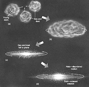
Another
consequence of rotation and angular momentum is the flattening
of clouds into a single plane that sit perpendicular to the axis of primary
rotation. This process is also believed to be the method for flattening
galaxies (as seen to the right). When particles in the system come closer
together as the cloud contracts, the conservation of angular momentum will give
each particle more kinetic energy as it swings about the centre of mass (just
as ice skaters increase in rotational velocity as they retract their extended
arms). The particle’s rotation is really only pronounced about the one primary
axis. Thus the particles in the plane central to the axis will move faster, but
their high tangential velocities will prevent them from being sucked into the
centre of mass because their centripetal acceleration will be relatively small.
The particles above and below this plane will be drawn more in toward the
centre, feeling the pull increasing out to the poles of the system. They
experience a greater force that will more easily overcome their slower
tangential velocities (their rotational momentum about the axis will decrease).
The result is the concentration of the cloud (whether it be of multiple system
or not) into a planar formation.
The
‘squashing’ of clouds into such planes has no effect on the development of the
star. In fact, the process seems inevitable. The envelope will continue to bear
down on the protostar’s core while it accretes matter. The planar alignment of
the accretion disk is important in understanding the reversal of the accretion
flow as the star ignites and blows the remaining matter cloud back into the
ISM. This process is known as the outflow and will be looked at in the next
section.
The
one hindrance angular momentum does have on a collapsing system is its increase
of the total kinetic energy in the system. If the total KE becomes too high,
the cloud will naturally withstand any more collapse by exerting pressure
against the gravitational forces. This is why the radiative cooling (releasing
the gravitational potential energy) of molecular clouds to low temperatures is
crucial in the early time of protostar development.
Taking
into account this slightly more complicated picture of stellar formation, one
of several question remains to be asked: what is the critical mass of a cloud
that will allow gravitational attraction to over come the forces of the gases
trying to expand it? An estimate for this critical mass, known as Jean’s Mass
(MJ), in a matter cloud can be calculated with the equation below:
where
‘T’ is the cloud temperature, ‘r’ is the density, ‘mH’
is the mass of a hydrogen atom and ‘m’ is the mean atomic weight
of the cloud relative to hydrogen.
This
equation concerns the entire massive cloud, not the individual molecular
clouds. A cloud above Jean’s Mass should eventually fragment into smaller
concentrations, which should ultimately develop new protostars.
As
the extent of fragmentation can vary considerably across one massive cloud,
certain experimental calculations have shown that the lowest possible mass of
one collapsed sub-cloud region is about 10MJ. The instabilities in
the massive cloud’s collapse can result in a whole range of different stars and
multiple systems. It is believed that those stars that have a chance of forming
a planetary system would have masses up to 15MJ. There has been
discussion over the importance of low mass brown dwarf stars
(considered as failures of star formation)
and their relevance to stellar formation theories. It is suggested that any
object of a mass less than 10 MJ, accompanied by other stars in a
single cluster, would probably be some of sort planet. Brown dwarfs are thought
to have approximately the same mass, so the discovery of such a star isolated
in a collapsed cloud could present serious implication for formation theory: it
is not conceivable that contraction of molecular clouds, of greater mass than
their future protostars, could create anything less than a single very low
solar-mass star. If isolated brown dwarfs are found, their presence begs the
question of how they were able to form in the first place, or more precisely:
how nuclear fusion did not start given a quantity of matter more than
sufficient to cause collapse and heating to ultra-high temperatures.
What
is the duration now of the entire process of formation, with the latest forces
added? With multiple fragmentations, which could fragment themselves, the
length of time still depends of the amount of mass that accumulates in the
collapsing cores. If a massive protostar accretes enough matter, it will enter
the main sequence in as little as several hundred thousand years. If a cloud
has enough rotation, it will fragment normally (the condensation forming a low
mass protostar that may take several billion years to mature).
COMPLICATIONS – Magnetic fields and outflows A-2
Magnetic fields that
thread through the ISM are proposed to play a significant role in protostar
formation just as angular momentum does. Although angular momentum does
accentuate rotational motion of a cloud core, cores typically do still turn
quite slowly due to their considerable size and to, as it is suggested,
magnetic fields, which provide a ‘braking action’.
The magnetic fields of
developing protostars would form from the core and extend out through the
envelope. They are important in the two phases of matter accretion and cloud
dispersal. During accretion, the braking effect would ensure that the core is
rotating with nearly the same angular velocity as the envelope, ensuring that
there exists a sufficient quantity of matter that can easily be accreted about
the protostar. If the envelope rotated with greater angular velocity, the
accretion disk would evolve at a much slower rate and the protostar’s core
would not be able to take in as much in-falling matter. The same concept
applies to the formation of planetary systems around the future star: the
magnetic fields would slow the circumstellar matter down allowing it to
coagulate into sizable protoplanets12.
Magnetic fields may also
be a factor in the apparent overall inefficiency of star formation. Such a proposal
involves the ‘slippage’ of the neutral atoms and molecules of a protostar’s
circumstellar cloud and envelope through the slightly ionised components of the
same cloud, which are being held in place by a background magnetic field23.
The rationale is that such slippage in molecular clouds around developing
protostars pushes much of the matter back into the ISM – matter that could have
contributed to core collapse. It is possible that this might be a solution to
the brown dwarf problem if ever it is encountered: perhaps too much mass is
lots through slippage to sufficient densities cannot build up in the
protostar’s core to trigger nuclear fusion.
In a similar fashion,
magnetic fields seem to aid in the dispersion of the remaining envelope once
the protostar is nearing the main sequence. Observations of molecules around
candidate developing protostars reveal a fast bipolar flow away from the core
and envelope. This means that particles travelling at about 100km/s are being
pushed away  from the protostar in two opposite directions, collimating out of the
plane of rotation (up along the poles). The directions of the flows have been
inferred from bipolar Doppler shifts (both blue and red shifting) of the
high-speed particles moving with ‘forward’ and ‘reverse’ velocities. These
particle flows, which extend to a few light years, are estimated to carry a
considerable mass of ambient matter away from the protostar (see above image).
For such a distance, an enormous amount of energy must drive the lobes: they are
thought to be associated with the birth of a massive star, though the exact
source is unknown. It is worth noting that the bipolar flows have attracted
much interest, as it is such a process (though of a much larger scale) that is observed around extragalactic
compact radio sources. Mystery still surrounds the identity of the energetic
sources driving those clouds too. Promising scenarios for massive protostars
involve using the rotational energy stored in either the newly formed protostar
or its disk-like envelope, and strong magnetic fields to effectively act as a
giant fan that forces out the circumstellar gases. This picture might also be
coupled with the strong solar winds that would be channelled toward the poles
by the circumstellar disk (which is much more dense in the rotational plane).
The initial stages of this process probably would be hidden from view by the
surrounding gas and dust – but once enough matter has been pushed out and lobes
begin to form, they show up most brilliantly in the radio range of the
electromagnetic spectrum.
from the protostar in two opposite directions, collimating out of the
plane of rotation (up along the poles). The directions of the flows have been
inferred from bipolar Doppler shifts (both blue and red shifting) of the
high-speed particles moving with ‘forward’ and ‘reverse’ velocities. These
particle flows, which extend to a few light years, are estimated to carry a
considerable mass of ambient matter away from the protostar (see above image).
For such a distance, an enormous amount of energy must drive the lobes: they are
thought to be associated with the birth of a massive star, though the exact
source is unknown. It is worth noting that the bipolar flows have attracted
much interest, as it is such a process (though of a much larger scale) that is observed around extragalactic
compact radio sources. Mystery still surrounds the identity of the energetic
sources driving those clouds too. Promising scenarios for massive protostars
involve using the rotational energy stored in either the newly formed protostar
or its disk-like envelope, and strong magnetic fields to effectively act as a
giant fan that forces out the circumstellar gases. This picture might also be
coupled with the strong solar winds that would be channelled toward the poles
by the circumstellar disk (which is much more dense in the rotational plane).
The initial stages of this process probably would be hidden from view by the
surrounding gas and dust – but once enough matter has been pushed out and lobes
begin to form, they show up most brilliantly in the radio range of the
electromagnetic spectrum.
The final outflow
component is thought to be a jet of ionised particles that shoot straight up
and down from the protostar to a length of perhaps 1010 kilometres
at speeds reaching 300km/s (seen in image on the next page). The strong
magnetic field lines flow up through the accretion disk in the same direction
(though it bends in, then away, as it approaches, and leaves, the envelope).
The magnetic fields push along a molecular outflow at perhaps 50km/s that
surrounds the ionised ‘lane’ through its centre. Essentially the toroidal gas
volume around the protostar has two warped molecular cones coming off either
side.
If the influence of
rotation and magnetic fields is set out as ‘realistically’ as possible, being
correctly accounted for, the radiative spectra emitted from many candidate
protostars may provide verifiable support for this extended model.
The next series of
questions lie in the formation of planetary systems. The presence of the vast
outflows strongly alludes to the large circumstellar disks containing solid
matter (the disks have never been directly observed as they as blanketed with
dust). Once the majority of the envelope has dissipated, this leftover debris
may end up becoming the building blocks of protoplanets and eventually an
entire solar system. For example: a star in our galaxy, known as Beta Pictoris,
appears to be encircled by a disk of dusty material extending 6x10¹⁰km
from the star – planets may have already formed here. Another star, the famous
Vega that is around one-fifth of the Sun’s age, has once been the focus of a
study with IRAS. The results showed that there is a nearby cool cloud
170 AU wide of about 90
K, whose dust grains are about a thousand times larger than those typically of the
ISM. In total, these grains would be equivalent to 1% of the Earth’s mass.
Considering the star’s young age, the cloud might be a possible site of
planetary formation.
COMPLICATIONS – Galactic links: Shock
waves and
self-sustaining
star formation A-2
So
far, the models have centred on individual stars and clusters. Star formation
in matter clouds is very much a collective occurrence. This is where the models
enlarge in scope and incorporate processes of galactic proportions.
Firstly,
the contraction of molecular clouds is thought to be offset not only by
gravitational collapse, but also shock waves (‘density-wave patterns’)
that spread through the ISM. As a shock wave passes through matter clouds that
are significantly dense, the sudden pushing together of the cloud from the side
of the propagated compression wave can induce the gravitational collapse of the
cloud. If the conditions are right, an immediate shock front will cause the
cloud to contract and events to proceed as previously considered. The
triggering of these shock waves is attributable to a few known events: the
expansion of H II regions around young, especially massive stars (as in image
below) and supernovae explosions.
 As young OB-class stars ionise the
circumstellar gas and form an H II region, the heated gas expands back into the
neutral H I area. This ‘ripple effect’ creates a density-wave pattern that
moves outward through the ISM and develops the forceful shock fronts in dense
molecular clouds.
As young OB-class stars ionise the
circumstellar gas and form an H II region, the heated gas expands back into the
neutral H I area. This ‘ripple effect’ creates a density-wave pattern that
moves outward through the ISM and develops the forceful shock fronts in dense
molecular clouds.
The
same wave process applies to supernovae explosions. The sheer magnitude of such
an event is sufficient to propagate similar waves and tilt the gravitational
balance for molecular clouds. They may even trigger other supernovae explosions
in super-massive stars that are nearing the end of their shorter lifetimes and
are situated along the wave front.
The
‘chain reaction’ of a star formation can be regarded as the ‘sequential
feedback model’ and is prominent in massive cloud complexes. Cloud complexes
are usually in the shape of spheres, quite elongated along one axis. As star
formation sends out shock waves from one end of the cloud, a sequence of
formation events should follow in the shock front’s wake. New OB-class stars in
small sub-groups are born approximately
1
millions years after each density-wave pattern passes their dense molecular
cloud.
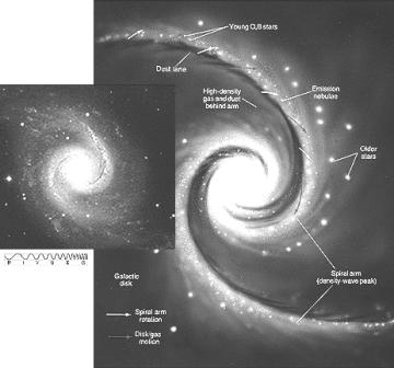 Now, in taking the viewpoint from an entire
galaxy, the representation of collapsing molecular clouds forming
protostars seems to have much in common with the way galaxies probably formed
in the past (for example: they form in one massive disk and have an axis of
rotation). During these times, star formation would have been much more
efficient and widespread. Today, the greatest amount of star formation seems to
take place along the each spiral arm’s boundary in spiral-armed galaxies (as
can be seen in the image to the left), especially if they are rotating at a
considerable rate. The ISM throughout the spirals arms of such galaxies looks
as if it is the densest compared to all other parts. As spiral arms rotate,
gases will be compressed in ‘spiral density waves’ and star formation will be
stimulated. Self-perpetuating stellar formation occurs when massive clouds in
the ISM are dense enough and shock fronts are in abundance.
Now, in taking the viewpoint from an entire
galaxy, the representation of collapsing molecular clouds forming
protostars seems to have much in common with the way galaxies probably formed
in the past (for example: they form in one massive disk and have an axis of
rotation). During these times, star formation would have been much more
efficient and widespread. Today, the greatest amount of star formation seems to
take place along the each spiral arm’s boundary in spiral-armed galaxies (as
can be seen in the image to the left), especially if they are rotating at a
considerable rate. The ISM throughout the spirals arms of such galaxies looks
as if it is the densest compared to all other parts. As spiral arms rotate,
gases will be compressed in ‘spiral density waves’ and star formation will be
stimulated. Self-perpetuating stellar formation occurs when massive clouds in
the ISM are dense enough and shock fronts are in abundance.
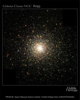
The
frequent development of stars in the past is suggested to influence the
formation of galaxies. Stars would form during the creation of a galaxy, and
any stars finding themselves outside the galactic plane would probably form
globular clusters as we observe them today. All other stars would normally form
open clusters inside the main disk and be carried in it as it rotates. Some
numerical simulations have proposed galaxies that did not have any spiral bars
to begin with, would eventually form some through the interaction of stellar
orbits18 – quite a claim indeed, something that may  never be verified.
Other
simulations have caused revision of theories involving the formation of
elliptical galaxies. The traditional notion was these galaxies formed from gas
clouds that did not have much initial rotation. Recent models say they could
have formed through collision with other galaxies. What is intriguing about
this model is the explosion in star formation, triggered by the unbelievable
shock waves created by such a catastrophic event. This would most likely use up
the vast majority of available gas too. As elliptical galaxies do not have much
gas at all or any
spirals that could encourage the formation of new generations of stars,
stagnation would occur (as presented in the graphs of Star Formation Rate – SFR
– versus time in the image above). This idea corroborates with the observations
that such galaxies are very old. Also, in dense super-clusters of galaxies, the
average counts of ellipticals are higher than spirals. The simulation regarding
the collision of galaxies to form ellipticals is supported by this observation,
as the era of galaxy formation would have been slightly lacking in empty space
with protogalaxies flying about in every direction (so the chances of collision
and hence elliptical galaxy formation would have been much higher).
Lastly,
what of the question concerning changes in formation processes of the first
stars during the universe’s Dark Ages, compared with the ones we model today?
 The simplest remedy to this mystery is a
slightly altered initial sequence of events that lead up to the same processes
of the current model. During the era of galaxy formation, there obviously would
not have been any galaxies in which stellar formation could have been stimulated
by shock waves in the ISM. The simple remedy is to assume that after a certain
period of time, a number of gas clouds had already coagulated, were
self-gravitating and moved about in space. When two gas clouds would collide
and form one, they would produce their own shock front
(as shown in the diagram above). This compression would act in the same manner
as the current model suggests: it would trigger star formation in the new
larger cloud by offsetting the gravitational collapse of denser cloud cores.
The simplest remedy to this mystery is a
slightly altered initial sequence of events that lead up to the same processes
of the current model. During the era of galaxy formation, there obviously would
not have been any galaxies in which stellar formation could have been stimulated
by shock waves in the ISM. The simple remedy is to assume that after a certain
period of time, a number of gas clouds had already coagulated, were
self-gravitating and moved about in space. When two gas clouds would collide
and form one, they would produce their own shock front
(as shown in the diagram above). This compression would act in the same manner
as the current model suggests: it would trigger star formation in the new
larger cloud by offsetting the gravitational collapse of denser cloud cores.
 These new stars would then form the building blocks of protogalaxies,
which would inturn create new stars, leading to the evolution of large-scale
structures in the observable universe and the current model of stellar
formation.
These new stars would then form the building blocks of protogalaxies,
which would inturn create new stars, leading to the evolution of large-scale
structures in the observable universe and the current model of stellar
formation.
An
extraordinary amount of new theory is being generated that somehow, or another,
incorporates stellar formation. Whether it is a theory on the nature and
effects of dark matter or super-massive black holes inside galaxies, star
formation seems to play a part, either in theory or in practise. This reaffirms
the notion that the stars are fundamental to all structures in the universe. In
this section, a few of the prominent theories that deal with more recently
extended stellar formation models will be visited.
Low-surface-brightness
(LSB) galaxies have been the focus of studies that suggest they collapsed and
formed at a later stage than the majority of conventional galaxies. Their blue
colour, a typical indicator of active star formation and relative galactic
youth, is difficult to understand. Measurements performed with radio telescopes
show they have rather low densities of neutral hydrogen gas. This and other
data support the idea that the surface gas density in a developing galaxy’s
disk must be greater than a certain threshold for widespread star formation to
occur.
The Schmidt Law states that the SFR of a spiral galaxy depends on the disk’s
gas surface density. LSB galaxies, it seems, might somehow stay below the
threshold value for a much longer time than conventional galaxies.
Another
theory proposes that the formation of galaxies and quasars is heavily
influenced by super-massive black holes. It has run into some trouble because
of the historical evidence showing a distinct time difference between stellar
formation and the beginnings of quasar activity.
The black hole theory proposes that the formation of the first ‘bludge’ in a
galactic disk, which would already contain developing stars, coincides with the
‘quasar phase’, which is, by its reasoning, the appearance of a black-hole
surrounded by a galactic bludge in the centre of the galactic disk. The
historical evidence contradicts this by saying that these two stages could not
have occurred simultaneously. This scenario is still “sketchy” and more
observations are required to make revisions. The theory’s main failing point is
its inability to explain what caused the ‘seed’ black holes to initiate the
whole process in the first place.
The
influence of dark matter on stellar formation has also received considerable
attention. Many different theories exist that propose stellar formation in
strange circumstances, in many ways unlike what the standard model of stellar
formation predicts.
One
of the chief reasons behind dark matter’s ‘existence’ is to explain
gravitational effects manifested in the motions of disks in galaxies, for
example. The problem is that luminous baryonic matter alone cannot be held
accountable for the observed effects. Regardless of whether dark matter is cold
or hot, is made up of Weakly Interacting Massive Particles (neutrinos, axions,
etc) or Massive Astronomical Compact Halo Objects (black holes, white and brown
dwarfs, etc), one of its fundamental features is to interact with normal matter
through gravity. Yet gravity is the very force that causes molecular clouds to
collapse and form protostars. So in the broader sense, it might be possible to
claim that the SFR is infact higher than what it would be without the universal
presence of dark matter, because dark matter (if it really does exist) would be
adding to the forces promoting cloud contraction and thus more stellar
formation.
Other
more detailed theories have been created involving the increase of the SFR in
protogalaxies due to non-baryonic dark matter acting as a ‘quantum fluid’,
which could condense in the absence of gravity.
As an over-dense region of ordinary baryonic matter and non-baryonic dark
matter would begin to collapse in the development of a protogalaxy, the dark
matter would condense into this quantum fluid. Tidal interactions with other
protogalaxies cause vortices to form in the quantum fluid, which itself does
not rotate about the protogalaxy’s centre of mass, as it does not directly
interact with the baryonic matter. The vortices create wells into which ordinary
matter falls. Once in these wells, the baryonic matter loses its angular
momentum, so in effect, it rapidly accumulates. This sudden increase in density
throughout the vortices will trigger large counts of stellar formation events
across the protogalaxy.
The
discovery of specific types of baryonic dark matter (the large number of white
dwarfs in the halo of our galaxy,
for example) seems to have serious implications, again, on theories of stellar
formation processes in the early universe. Current estimates show that in the
visible universe, stellar formation produces much more stars of lower mass than
of higher mass. However, the existence of a number of ancient white
dwarfs (with many more predicted to exist) suggests that in the early stages of
galaxy and star formation, the trend was reversed: many more massive stars were
created and than solar-mass stars.
The reasons for this are unclear at present – it is one of stellar formation
theory’s main mysteries.
Many
computer simulations have been run with varying initial conditions and
distributions of normal and dark matter to investigate galaxy formation.
Recently, increasing attention has been paid to the effects of star formation
and supernova feedback in such simulations. The aim of one simulation performed
in 2001, which incorporated all of these effects, was to resolve the “Angular
Momentum (AM) problem” found in previous simulations.
The problem arose from excessive transport of angular momentum from baryonic
gases to dark matter in the disk of the modelled galaxy, especially during
‘mergers’ with other galaxies. This simulation was found not to suffer a
devastating loss of angular momentum and the results reproduced many of the
fundamental properties for observed galaxies. The article addressing the
simulation results raises several pertinent issues associated with
computational modelling of CDM systems. It mentions another group of
researchers who argue, “that the inclusion of star formation can help stabilise
disks against bar formation and subsequent AM loss”. These bars are those
discussed previously, occurring in the earlier fragmentation simulations.
However, it seems with the inclusion of dark matter into the system, these
anomalies are largely overcome. Another issue raised states “it is not
currently possible to model individual star formation and feedback events in
cosmological simulations of disk formation”. The basis for this impossibility
depends on the modelling software and simulation parameters. In this case,
there was too greater difference between the timescales of supernova feedback
and the minimum time step of the simulation. These events were approximated so
that “each gas particle carries an associated star mass and can spawn two star
particles, each half the mass of the original gas particle”. This manner of
effectively approximating physical processes to one quantity or body is the key
in creating a successful simulation that can run efficiently on simulation
software – this will be reiterated in the project’s next part.
DEFINITION OF THE PROBLEM B-1
Unfortunately,
due to our position on Earth and the current capabilities of observational
equipment, directly viewing a small snapshot of a star formation event is
practically impossible. As has been shown while discussing the observational
clues that we can gather from massive protostar development, the radio,
ultraviolet and infrared emissions associated with stages in stellar formation
are only vague signposts and do not provide astronomers with the detailed
evidence required for significant advances in formation models. Thus
theories of possible models are developed using mainly inferences from
observations. Once they seem reasonably within the limits of a system, they are
‘put to the test’ in computer simulations to investigate the extent to which
they agree with predictions. Simulations on computers are helpful because
modelling software today is highly flexible and can take into several different
effects that may have a crucial impact on formation theory (even though it may
end up being a step in the wrong direction).
Despite
the fact that computers are still limited in speed, processing power and
storage space, professional simulations are run with highly optimised
algorithms on parallel-processor supercomputers. One of the most common
algorithms incorporates complex ‘Smoothed Particle Hydrodynamics’, or SPH,
equations, which provide an efficient way of calculating particle dynamics in a
many-bodied system. The actual modelling of individual particles in a molecular
cloud, for example, is far from an achievable reality because the sheer number
of bodies is too great for any configuration of computers to handle. Therefore,
single particles can be approximated to exist in larger bunches: a group of
particles is treated as one ‘quantity’ so that calculations may proceed at an
optimal rate without incurring severe mathematical errors on the properties of
imagined individual particles. The calculations are performed so that the
effect of a single quantity of particles is taken into account throughout the
entire system. This is part of a typical scenario in simulating an “N-body”
system (known this way because the system contains any number of particles).
The need for an analytical approach in calculating system dynamics results from
the “N-body problem” encountered in continuous analysis. The problem states it
is impossible to take into account the effect (the forces, etc) of more than
one particle on another single particle simultaneously (in one instant
of time of the system itself). This constraint arises because in the moment
that the effect one body has on another is calculated, the third body would
respond to those same forces and change position (if the focus was on each
body’s displacement). That is to say: if a system contains only two bodies,
calculation of both bodies’ effect on the other in one mathematical function,
for one instance of time, is easy. On the other hand, if there are three or
more bodies, it is not possible to do this because as the mathematical
calculation is performed for two particles, the others will alter in their
properties. To overcome this, the analytical approach is necessary. It involves
stepping through each body and applying its effect to every other body. In this
way, it is not necessary to consider performing continuous integration of the
mathematical functions governing each body’s dynamics in sequence. The valid
option in this analytical approach is to make the system perform as a function
of an independent variable (usually time). With time, its value is incremented
for each frame (or ‘snapshot’ of the system) and the simulation calculates each
body’s effect on every other body as a function of the last time increment.
This is fundamental analytical procedure used in the vast majority of N-body
simulations, and although it does not match the real world’s ability to
overcome the N-body problem, it provides a sufficiently accurate representation
of physical events, based on a system’s constants and initial conditions.
Many
N-body simulations have been performed for the collapse of galaxies, now
especially inclusive of the Cold Dark Matter theories. As mentioned previously,
such modelling has attempted to incorporate the influence of stellar formation
and supernovae explosions in developing galaxies. Fewer simulations have been
performed on star formation events themselves. The second part of this project
deals with putting the simpler ideas of stellar formation theory through
simulations in order to investigate the changes in development caused by
altering initial conditions, the numbers and types of particles, distributions,
initial velocities and rotation, and selecting different combinations of
effects (for example angular momentum and radiation pressure). By comparing the
outcome of each simulation, it is possible to obtain a better understanding of
the influence each effect and condition has on a system, and hopefully promote
further thinking to extend the current models in the right direction.
Naturally,
to perform any calculations of particle dynamics on a computer, modelling
software must be written to handle such simulations. Some of the hallmarks of
any good multipurpose modelling package is its ability to live up to increasing
computational demands, incorporate relatively hassle-free extension including
more procedures and physical effects, and scalability and compatibility on
newer, more sophisticated software and hardware platforms. As part of this
project’s investigation of very simple stellar formation models, I have
attempted to write my own modelling software to perform the simulations. The
irony is, considering the current state of the software and my own relatively
basic mathematical, physical and programming knowledge (compared to those
scientists who design SPH modelling software for parallel-processing
super-computers), the software does not exactly measure up to any of those
hallmarks. Not only this, but the relatively late fruition of my ideas
inspiring me to attempt such a task, has not left enough time to fully complete
all components of the software. It is operational, however experiences very
limited functionality.
The
purpose of my software and rudimentary model inclusion into the project is
two-fold. On one hand, to look briefly at the scaled-down process of creating
modelling software and writing the physics and mathematical calculation
procedures. On the other hand, to discuss ways of approximating known stellar
formation theory and choosing the model’s crucial assumptions in order to
perform some simulations.
Firstly,
I shall give a concise overview of the modelling software. It is designed to
operate on workstations running the Intel hardware and Microsoft Windows
software platform (compatible versions are Windows 98, Me and 2000). Although
the software can run on one computer alone, its primary feature is the
distribution of the computational workload. To take advantage of this, the
software can be loaded onto as many computers as there are connected to a
network. It is even possible to extend this configuration from a simple Local
Area Network, to a Wide Area Network – the software communicates in the same
manner, though speed factors may come into play on WANs such as the Internet.
The software does not support multi-processor systems as yet – it will be a
future improvement: calculations will be spilt and allocated to different
‘threads’ running on separate processors, increasing the speed by a factor
roughly of the number of CPUs.
The
modelling software consists of several components, each contributing varying
degrees to it’s functionality. The main components are the ‘Marshaller’ and
‘Worker’. The Marshaller is used to set the initial conditions, effects and
parameters of the simulation. The Worker software is installed on each of the
networked workstations and performs the actual simulation calculations. Other
components are the ‘Plugin Host’ (this is a Windows NT ‘Service’ that runs as a
Dynamic Link Library housing for ‘plugins’, such as the Worker software, that
have been created with conventions I have specified) and ‘Plugin Host
Configuration Utility’ (which enables the remote installation and control of
the Plugin Host on each workstation – for example, it overcomes the problem of
manually installing the software onto each workstation, by automatically
connecting to each one and configuring them remotely). The final component is
the extension for both the Marshaller and Worker: the “Effects”. Effects are
also plugins that are used to apply any sort of force or effect to bodies in
the simulation – this will be discussed again shortly.
Once
the workstations are running the Worker software, a new simulation can be
created in the Marshaller. The available Workers can be added to the
Marshaller’s Worker selection list – the selected workers will handle the
calculation of the simulation. The next step is to specify the initial
conditions and parameters of the simulation. At the moment, the set parameters
that can be controlled are: initial velocity, initial distribution, system
lifetime and particle types. Each of these parameters has extended settings.
For example, the initial velocity can be set to zero, random directions,
rotation about a point along an axis, toward or away from a point or it can be
based on an ‘expression’ that is written using pseudo-algebraic terms (setting
the velocity for each particle as a function of its displacement is one
possibility). Similar options exist for the initial distribution (random
displacement in a sphere or box, functional distribution dictated by an expression,
filling a 3D object, even spacing or slight perturbation off even spacing) and
system lifetime (not fixed – so it stops on command, fixed: the simulation
finishes once a system is a specified age, or completion on the satisfaction of
certain criteria, such as attaining a critical particle density and confinement
for ignition of nuclear fusion). Multiple particle types can be specified. Each
particle has a unique count (or percentage of the total), mass and radius.
Particles can also have separate rules governing them as opposed to the global
initial conditions and parameters already listed. For example: it is possible
to have a total of 3 particle types and to specify that the global initial
conditions should govern 2 of them, but have a separate distribution pattern
for the third. The global conditions can also be applied to these
particle-specific settings, so that a combination of the two governs a particle
type’s behaviour (not just one or the other). If the user is satisfied with the
initial conditions and parameters, he or she can connect to each selected
worker and automatically transfer the initial conditions to each one. In doing
so, the Marshaller benchmarks each Worker to gain an idea of its processor
rating (how many calculations it can perform relative to the other Workers).
Once it has obtained a processor rating, the Marshaller then divides the total
number of particles up into sizable chunks, relative to a Worker’s processor
rating, for each Worker to handle (chunks that each Worker should finish at the
same time). When the user clicks on the ‘Start simulation’ button, the
Marshaller will send a ‘save, prepare and start’ sequence to each Worker. When
a Worker receives such a set of commands, it saves the current simulation
configuration (in case the user would like to resume a simulation later on or
continue one based on the conditions and state of another), prepares its
allocated section of the system and starts working.
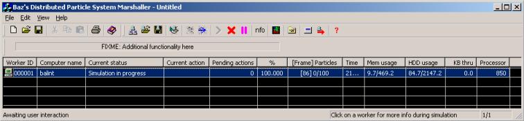
As can be gathered from the networked Worker approach, this is a distributed
style of computing. Therefore, the most important aspect of such distributed
simulations is to split the simulation up effectively and fairly, and then to
make sure each Worker has the correct information of the whole system through
the entire duration of its lifetime. The other consideration lies in the
analytical modelling method. In the end, the goal of the simulation is to
calculate the new displacements of each particle after taking into account any
forces acting upon them. To do this and overcome the N-Body problem, these
calculations must be done in sequenced ‘frames’ or ‘snapshots’, each with its
own system time. Thus the other factor set in the Marshaller’s initial
conditions it the frame time: the time increment between each frame of the simulation.
The options for this are: fixed increments, adaptive increments (if there is no
significant motion in the majority of particles then the increment is increased
until particles start moving at least a little – complex statistical analysis
must be implemented here to ensure mathematical errors do not occur in pushing
the increment value too high) and linear and accelerating increments. The
consequence of frame times in the distribution of calculations is that each
Worker must synchronise its particle system ‘snapshot’ (the properties, for
example: position and velocity, of every particle in the system) with
every other Worker so that the calculations may proceed correctly while every
Worker is calculating the same data. The issue of synchronisation comes into
play in the preparation and at the conclusion of calculation for each frame of
the simulation. When each Worker has finished creating its allocated
section of the entire particle system, it communicates this allocation to every
other Worker in exchange for their allocations. When synchronisation has
completed, every Worker will have the same snapshot of the entire particle
system on which to work. Once the Workers have finished calculating each
subsequent frame of the simulation, the synchronisation process starts again
until the simulation can continue. The future design of the software should
re-allocate the particle system across each Worker in the event that one or
more go ‘offline’ and disconnect from the simulation, which otherwise would cause
the simulation to abort.
The
one point that has not been mentioned so far is that in this developing example
of the simulation, nothing would actually happen to any particles because no
Effects have been configured to run with the simulation. As briefly stated, an
Effect serves as a force on each particle in the system and also conforms to
the modelling software’s modular architecture, making the software fully
extensible in this way.
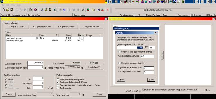
An
example of an Effect follows: the first one created was ‘Newtonian Gravity’ –
it calculates the attractive force in newtons between two particles and adds
the force vector to the particles’ resultant force vectors. The Effects are
initially configured on the Marshaller and each Effect’s custom configuration
data is sent to each Worker (which must have the same Effect installed too). As
each Worker calculates a frame of the simulation, it ‘realises’ the selected
effects on the specified particles. As with the global and particle
type-specific initial conditions parameters, so to can Effects be configured
globally and per particle (interesting results can come from changing the
Universal Gravitational Constant, especially on one type of particles among
other groups). Once each Effect has been realised on every particle, the Worker
cycles through each particle and applies the resultant force, which accumulated
for that one frame, to the particle: the force is multiplied by the particle’s
mass to give acceleration – this is then multiplied by the time increment for
that frame to give a velocity vector that is added to the particle’s current
velocity vector. The new velocity
vector of the particle is multiplied by time increment again to obtain a
displacement vector that is added to the particle’s current displacement, in the
end moving the particle. Any number of Effects can be created to calculate any
number of physical forces on a particle system, such radiation pressure,
collision handling and angular momentum.
In
terms of each Worker’s load, one Worker will only calculate the new
displacement for the particles that have been originally allocated to it. The
calculations do still take into account all other particles, but the
distribution of calculations is achieved by having each worker only process its
own particles in the context of the system.
The
distribution of calculations gives rise to any increase in overall
computational power of the Worker ‘collective’. The only concern for a
simulation is network speed and traffic conditions. The total size, in bytes,
of each Worker’s particle allocation is relatively small if there are quite a
few Workers and a moderate total particle count. So on a high-speed network,
the synchronisation stage of the Workers, following each calculated frame of
the simulation, should not take very long compared with the time to calculate
one frame itself. If there is excessive traffic on a large scale network and a
large number of Workers, the time difference between the two functions may not
be all that large, so the positive effect of decreased total calculation time
of the distributed approach is lost. Thus, care must be taken to configure the
network correctly, ensuring traffic is kept to a minimum and that a sufficient
amount of particles is chosen so that the benefits of distributed computing may
be realised (if too few particles are selected, the synchronisation time over a
large number of workers will again outweigh the calculation time, rending that
simulation inefficient).
At
the end of the simulation (regardless of whether is it ended, or the lifetime
criteria are met), frame data from each Worker is sent back to the Marshaller
to be reassembled into one continuous sequence. There exists a specific viewer
incorporated into the Marshaller that enables the user to view each frame of
the simulation in both 2D and 3D space. Density maps can also be created in
specific dimensions to demonstrate the desired dynamics of a system (for
example several images might be created to show the planar distribution of
particles in a system that had initial rotation and collapsed into a disk).
Unfortunately
due to time pressures, the software has not been finished. The only Effect that
exists is gravity and the synchronisation functions have not been completed (so
the simulation can only run on one computer). Also, as to be expected with any
software-under-development, the Marshaller and Worker need more debugging to
fix current problems and to prevent future ones from occurring. A test
simulation has been run to check if the basics of the Marshaller and Worker
run. Indeed the simulation frames’ viewer displays the image sequence and the
pictured particles do move due to the Effect of gravity – the software’s
functional prospects are ‘looking good’. Although the Worker’s calculation
algorithms are heavily dependent on that of each installed Effect, and do not
incorporate any advanced functions like those of SPH (in part because they are
out of my league at the moment), the software itself really only serves as a
little experiment in distributed computing and an easy-to-use tool for
simulating simple N-body systems and investigating the influence a combination
of physical forces (Effects) will have on a system’s development. This was the
philosophy behind its creation for this project, but because there has not
enough time to complete the software, design some more effects and actually run
the simulations, the original idea has not yet been fulfilled. It stands at the
moment as ‘work in progress’ and will be completed hopefully in the upcoming
months. I hope that this software package will have some sort of future as I
have spent much time and effort creating it and I would like to see some good
use out of it – even if it is only on small and simple scales.
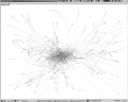
 The entire software package has been created over the last 3 weeks. It
has been written in Microsoft Visual C++ 6.0 and requires MFC 4.2 and newer ATL
DLLs than those found in NT 4. A count of the number of lines of code (of every
sub-project in the package: Marshaller, Worker, Plugin Host, Plugin Host Configuration
Utility and Effect prototype) yields a sum of about 13 000 (my biggest project
so far). It will continue to grow later in the year. Once it is fully
operational, I will perform the original simulations I intended for this
project and post the results, images and density maps on my website at http://homepages.tig.com.au/~balint
The entire software package has been created over the last 3 weeks. It
has been written in Microsoft Visual C++ 6.0 and requires MFC 4.2 and newer ATL
DLLs than those found in NT 4. A count of the number of lines of code (of every
sub-project in the package: Marshaller, Worker, Plugin Host, Plugin Host Configuration
Utility and Effect prototype) yields a sum of about 13 000 (my biggest project
so far). It will continue to grow later in the year. Once it is fully
operational, I will perform the original simulations I intended for this
project and post the results, images and density maps on my website at http://homepages.tig.com.au/~balint
Despite
the fact that I am unable to put any simplistic models through my software in
its current state, the possible models for the early part of a stellar
formation event deserves a short discussion.
The
object of testing different models is to discover what effect the differences
between them has on the overall system. As this project has gradually built up
the understanding of stellar formation, and in doing so has listed more and
more forces that, as it is perceived, come into play, it is the same rationale
behind gradually building up this simulation model.
The
goal of the models here would be to simulate an approximated molecular cloud
and add forces to investigate how its collapse is affected and whether a
protostar could have the chance of forming, and maybe later seeing whether
fusion ignition could be reached (through satisfaction of the Lawson criterion
governing the minimum density-containment time of particles in plasma, required
to start self-sustaining fusion reactions).
The
first step is to identify to what extent molecular clouds should be
approximated to make the simulation’s calculations efficient, while still
retaining physical accuracy to the real physical event as much as possible.
This means, instead of accounting for every single particle in a
molecular cloud (which is huge), a group of several particles would be
treated as one big ‘particle’ by the simulation. Thus one ‘particle’ would have
the many, many times mass and radius of one dust grain or hydrocarbon. The
collisions of particles (an Effect that would be activated at a later stage)
would have to randomised too, as just because one ‘particle’ overlaps another’s
space, the bodies inside them may not be touching. However another
consideration is radiation pressure and the extent to which it will counteract
the force of gravity. Collisions are necessary to convert kinetic energy into
radiation, which inturn would increases the radiation pressure as the system
heats up. So a balance between the two must be struck, and several simulation
test runs might be dedicated to investigating this.
Yet
another Effect that would have a significant influence is angular momentum.
This would be another crucial step in understanding what influence is has on
such a collapsing system. If the parameters are realistic and the Effects’
influence proceeds as planned, it would be very rewarding to see clouds both
fragment, form increased concentrations of mass, which would inturn collapse
and form an envelope. If these series of events were to occur, it would show
that the model was reasonable correct. If not, the model may require some
‘tweaking’ or be completely incorrect (with a bit of luck it is not the
simulation software itself). This very process reflects the ordeal professional
astronomers and cosmologists go through in taking observational evidence,
analysing probable models tested in simulations, and then attempting to create
newer, more accurate models that fit all available knowledge. This is the very
core of the scientific method itself.
Once
a model has been simulated here and different combinations of Effects have been
tested, analysing exactly what each Effect has, and what the general results
were, would be satisfying and enlightening, while also reaffirming of the
theory. Although improvements to the simple model here may be necessary anyway,
but are too complex to be handled by the simulation, it would still give a
sense of the process of reviewing models and suggesting well-founded theories
that could be the solution to a more accurate and improved model for the
future.
This picture is taken from the analysis of simulation
results of galaxy
formation with star formation feedback and is the kind
of output
the Marshaller will give. The software used here was
GADGET.
(http://www.mpa-garching.mpg.de/gadget/sfr)
Stellar
formation is one of the most essential, yet primal, events of the cosmos’
construction and evolution. Stars are the main component of galaxies; stars
process lighter elements and create heavier ones that form the dust and gas of
the interstellar medium; stars create planetary systems and provide energy to
life that may inhibit such homes; stars form in different configurations and
have lifetimes with alternative endings: some die and cool slowly, others
explode in spectacular flashes – all this from a ball of plasma. The formation
of stars was crucial to the evolution of the universe. In humanity’s yearning
to understand the universe, astronomers have made several key observations and
used computer simulations to at least try and predict how these sparkling orbs
come about. Its complexities are still another mystery, intertwined with galaxy
formation and dark matter. With the progress that has been made in current
stellar formation models, it would be pleasing to see the theory mature
alongside new observational evidence provided from radio and infrared
telescopes – a great deal is in store for SIRTIF. So much attention has been
drawn to developments in the evolution of large-scale structures in the
universe – if good progress is made in the future, awareness of such a key area
as in-depth star formation will increase. A better understanding of the
processes involved in star formation, and the effect on its surroundings,
promises to have consequences, not only for other theories, especially
regarding galaxy formation, but also perhaps for the very fundamentals that we
perceive to dictate the physical universe.
Creating
a simple model of the early stages of stellar formation seemed like an
interesting application of the knowledge I have gained from researching this
project. Despite the forward push of time and the looming HSC, I was unable to
test the with my incomplete simulation software. However, all things
considered, I believe this has been a fulfilling, beneficial and fun
experience. I would like to continue this project once I finish school: I plan
to finish the simulation software and write a wide variety of Effects to
combine. I guess I shall taste the world of professional astronomers and
programmers who attempt to perform these miracles on a regular basis. I will be
able to put the many forces governing stellar formation to the test, to really
see and exemplify what effect they have on protostar development – what really
might be going on in the intangible interstellar medium.
·
Encyclopaedia
Britannica, Multimedia Edition 1999 (CD-ROM):
o
The
Interstellar Medium (Article)
o
Galaxies:
Dust clouds
o
Galaxies:
The general interstellar medium
o
The
Cosmos – Star and Chemical Elements: Star Formation
·
Scientific
American (http://www.sciam.com):
o
Bothun,
G.D., The Ghostliest Galaxies”, March 1998
o
Musser,
G., “The Whole Shebang”, October 2000
·
Parker,
B., “Creation”, Chapter 4, Plenum Press, New York, 1988
·
Harrison,
R., “Cosmology”
·
Zeilik,
Michael, “Astronomy: The Evolving Universe”, John Wiley & Sons, 1988
·
Meadows,
A. J., “Stellar Evolution”, 2nd Edition, Pergamon Press, 1978
·
Lightman,
A. and Brawer, R., “An Introduction to Modern Cosmology”, Chapter 1, “Origins,
The Lives and Worlds of Modern Cosmologists”, Harvard University Press,
Cambridge, Mass, 1990
·
Thickett,
Geoffrey, “Pathways to Chemistry”, Macmillan Education Australia, 1996
·
Rickey,
Tom, “The Rochester Review”, University of Rochester, New York, 1999, “The Last
Great Eye in the Sky” (http://www.rochester.edu/pr/Review/V61N3/feature4.html)
·
Thinkquest,
“Life Cycle of Stars”, 1998 (http://library.thinkquest.org/17940/texts/star/star.html)
·
“Dark
Matter, and the Formation of Galaxies”
(http://www.usm.uni-muenchen.de/people/botzler/lecture/lect.html)
·
Astronomy
- Studies of the stars - Studies of the Universe, “Stars”,
(http://www.st-and.ac.uk/~www_pa/personal/rwh/as1002/starsi.pdf)
·
Leicester
University Astronomy Group, “Brown Dwarfs & Stellar Formation”, 1998. (http://www.star.le.ac.uk/astron/brown/contents.html)
·
“Galaxy
Formation” (http://zebu.uoregon.edu/~js/ast123/lectures/lec28.html)
·
“Lawson
Criteria for Nuclear Fusion”
(http://hyperphysics.phy-astr.gsu.edu/hbase/nucene/lawson.html)
·
“Star
formation and feedback in isolated disk galaxies”
(http://www.mpa-garching.mpg.de/gadget/sfr)
·
“Cosmological
Dark Matter: An Overview” (http://www.astro.ucla.edu/~agm/darkmtr.html)
·
The
Astrophysical Journal, 555:L17-L20, 2001 July 1: Thacker, R.J., Couchman,
H.M.P., “Star Formation, Supernova Feedback and the Angular Momentum Problem in
Numerical Cold Dark Matter Cosmogony: Halfway There?”
·
Science:
Onaga, L., “Astronomers detect elusive dark matter in Galaxy” (http://www.usatoday.com/news/science/aaas/2001-03-22-dark-matter.htm)
·
Berkeley
Campus News: Sanders, R. “Astronomers at UC Berkeley, Edinburgh, Cambridge,
Vanderbilt report first direct detection of dark matter in galactic halo, part
of universe's missing mass”, 22 March 2001 (http://www.berkeley.edu/news/media/releases/2001/03/22_halo.html)
·
Peoria
Astronomical Society: Ware, D., “PAS General Articles: Why Do Stars Form?” (http://www.astronomical.org/astbook/starform.htm)
·
‘Our
Sun’ (Title sheet): [Unknown] H II spectra photographed by SOHO
·
‘The
Star Cluster of M13’ (p. 6), ‘An Active Stellar Nursery’ (p. 18), ‘Initial Star
Formation Rates’ (p. 31), ‘Star Formation’ (p. 32),
‘Globular Cluster of M80’ (p. 32):
“Galaxy Formation” (http://zebu.uoregon.edu/~js/ast123/lectures/lec28.html)
·
‘The
Orion Nebula’ (p. 7): Encyclopaedia Britannica Online (http://search.ebi.eb.com/ebi/binary/0,6103,30589,00.gif)
·
‘Trapezium
cluster’ (p. 13): “Images of the Universe” (http://www.mv.cc.il.us/alternativelearning/starimages.htm)
·
‘Pleides
cluster’ (p. 21): [Unknown]
·
‘Gas
cloud collapse’ (p. 23), ‘Spiral Galaxy’ (p. 30): “Dark Matter, and the
Formation of Galaxies”
·
(http://www.usm.uni-muenchen.de/people/botzler/lecture/lect.html)
·
‘GADGET
Graphic Output’ (p. 46):
“Star formation and feedback in isolated disk galaxies”
(http://www.mpa-garching.mpg.de/gadget/sfr)
